A story of commutators

The conceptual step that took humans from their pre-conceived “classical” notions of the world to the “quantum” notion was the realization that measurements don’t commute. This means, as an example, that if you measure the position of a particle exactly, you cannot simultaneously ascribe to it an infinitely precise momentum.

This is not simply a statement about the ultimate accuracy of measurements. In fact, you can measure any one of these variables to as high a precision as you desire. The statement above represents a property of nature – the things that we call particles do not actually have an infinitely precise position and an infinitely precise momentum at the same instant of time. The simplest way to express that these (different observables like position and momentum) are “complementary” means of describing the results of measurements, is to represent observables as matrices. The possible results of measurements of these observables are eigenvalues of these matrices. In this language, states of the world are represented as vectors in the space on which the matrices operate.

Then, one can express the fact that one observable is not precisely determined if another one is, by requiring that the two matrices (that represent these observables) ${\bf NOT}$ commute. If you recall linear algebra from high school, two matrices that do not commute have eigenvectors that aren’t all the same. Suppose you have a precise eigenvalue for a state that is an eigenvector of one observable (i.e., a matrix). Since it isn’t an eigenvector of another (non-commuting) observable (i.e., another matrix), that state is not one that has a precise eigenvalue for the other observable. Said in this way, the construction automatically implies that the two observables are complementary – a vector cannot generally be an eigenvector of two non-commuting matrices at the same time.

This is the origin of the famous commutator that people start off learning quantum mechanics with, ${\it viz.} \:$

$[ x, p] = x p - p x = i \hbar$

Here, $x$ and $p$ are the position and momentum of a quantum particle and the order of the operators implies that if one applies the momentum operator to a state (“measuring” its momentum), the answer one gets for the position operator is different from what one gets if one reverses the order of the measurement. In fact, Heisenberg’s famous uncertainty relation is a direct mathematical consequence of this operator equation. In the above $\hbar$ is the redefined Planck’s constant $\hbar=\frac{h}{2 \pi}$ .

To repeat what I just said – to make sense of his uncertainty relation, Heisenberg realized that what we think of as ordinary variables $x, p$ are actually best represented as matrices – things people study in linear algebra. It is not common to have numbers that don’t commute. It is more common for matrices to not commute, where the order of multiplication of the matrices gives different resultant matrices. Matrices have eigenvectors and eigenvalues, so if a particle is (for instance) in an eigenstate of its position operator, then its position is specified to infinite precision. Its position is, then, the eigenvalue of the position matrix in that eigenstate.

The first non-trivial application of the (then) new quantum mechanical formalism was to the problem of the harmonic oscillator. This is the physics of the simple pendulum oscillating gently about its point of equilibrium.

${\cal E} = \frac{x^2}{2} + \frac{p^2}{2}$

Here $x$ is the position of the particle and $p$ is its momentum. This formula usually has constants like the mass of the particle and a “spring-constant” – I have set all of them to 1 for simplicity.

A Russian physicist named Vladimir Fock realized a cute property. If you define

$a = \frac{x +ip}{\sqrt{2 }} \\ b = \frac{x - ip}{\sqrt{2}}$

then, using the basic commutator for $x, p$ , we deduce that

$a b - b a = \hbar$

and the energy can be written as

$\frac{\cal E}{\hbar} = b a + \frac{1}{2}$

Now, a peculiar thing emerges. One can compute the commutator of $a$ and $b$ with ${\cal E}$ , the energy “operator”. One finds

$\frac{\cal E}{\hbar} b = b (\frac{\cal E}{\hbar}+1) \\ \frac{\cal E}{\hbar} a = a (\frac{\cal E}{\hbar}-1)$

The interpretation of the above equation is simple. If you apply the operator $b$ to a state of the harmonic oscillator with energy ${\cal E}$ , the new state that emerges has one more unit of energy, in units of $\hbar$ . The operator $b$ increments (or “raises”) the system’s energy (and hence changes the system state), while the operator $a$ decrements (or “lowers”) its energy by one unit of $\hbar$ (and hence changes the state).

This would have just been an interesting re-write of the basic equation of the harmonic oscillator, until the physicist Paul Dirac used this language to analyze the electromagnetic field. He realized he could re-write the electromagnetic field (actually, any field) as a collection of oscillators. He then interpreted photons, the elementary quantum of the electromagnetic field as the extra bit of energy created by a suitably defined $b$ operator for every oscillating wave-frequency. The quantum theory now expresses that the electromagnetic field can be described as a collection of identical photons, whose numbers can increase and decrease by 1, by the application of an appropriate $b$ operator. Interactions between the electromagnetic field and other particles basically involve an interaction term with a $b$ operator to create a photon. The photons are, in this picture of the world, regarded as the individual units, the “quanta”, of the electromagnetic field.

This is not just a re-write, therefore, of the basic energy function for an electromagnetic field. It is an entirely new view of how the electromagnetic field operates – so novel that this procedure is (for no apparent reason) referred to as “second quantization”. It solves the puzzle of why photons are all alike. They are all created by the same $b$ operator. And the operator $b \: a$ is called the “Number” operator – if there are ${\cal N}$ photons in the electromagnetic field, then it is an eigenstate of this “Number” operator, with eigenvalue ${\cal N}$ .

This formalism has been very fruitful in research into quantum field theory, which thinks of particles as the individual “quanta” of a quantum field. In this view, there is a quantum field for photons (a kind of boson that we interact with all the time with our eyes). There is a quantum field for electrons, a kind of fermion.

In fact, since photons are a kind of “boson”, the standard commutator for bosons is written as

$a b - b a = 1$

where the constant $\hbar$ is absorbed by suitably redefining the operators $a$ and $b$ .

Then fermions were discovered. It turns out that they are better described by the commutator

$a b + b a = 1$

Due to the plus sign, this is usually referred to as an anti-commutator.

The plus or minus sign might seem like a small alteration, but it represents a giant difference. For instance, a bosonic harmonic oscillator can have a countable infinity of states – corresponding to the fact that you can make a beam of monochromatic laser light as intense as you want by having extra photons in the beam. A fermionic harmonic oscillator (with the plus sign), on the other hand, only has two states – one with no fermion and one with one fermion. You cannot have two fermions in the same state, a fact about fermions that is usually referred to as the Pauli exclusion principle.

Let me now proceed (after this extensive introduction) to the topic of this post. It is meant to explain a paper I published in the Journal of Mathematical Physics. In this paper, I study particles in two dimensions, which have properties intermediate between bosons and fermions in a manner akin to how anyons (particles in two dimensions) behave. I wrote a rather long blog post on anyons here, which might be a simple introduction. While, people have studied particles with intermediate statistics, I studied (with a lot of very inspiring discussions with Professor Scott Thomas at Rutgers) the algebra

$a b - e^{i \theta} b a = 1$

The parameter $\theta$ is a constant and can be chosen to be some fraction of $2 \pi$ . I studied both rational and irrational fractions of $2 \pi$ . If we considered only rational fractions, then $\theta = 2 \pi \frac{M}{N}$ . It turns out that we can safely study the case where $M=1$ , as that covers all the possible rational cases well. In that case, notice that if $\theta=0, N = \infty$ , the resulting commutator corresponds to the case of a bosonic oscillator ( $e^{i 0} =1$ ). The case $\theta = \pi, N=2$ corresponds to a fermionic oscillator. Particles with intermediate statistics are represented by $N=3,4,5....$ .

Some results emerge almost immediately. The number of states accessible to a harmonic oscillator that obeys the algebra for $N=2$ (the fermion) is exactly 2. The number of states accessible to a harmonic oscillator that obeys the algebra for $N=\infty$ is $\infty$ . So, quite as expected, the number of states accessible to a particle described by the algebra for a general $N$ is, indeed, $N$ .

These states are described by an “energy” function that is a set of complex numbers on the complex plane. These complex numbers lie on a circle. For $N=2$ , there are only two points – its like a flattened circle. For $N=\infty$ , the eigenvalues lie of a line, which may be thought of as the perimeter of a circle of infinite radius. For intermediate values of $N$ , the circle has a finite radius that is bigger than 0.

The interesting part that emerges from this is an arithmetic and calculus that emerges from the algebra. Since $a$ is a matrix (in our picture), suppose we consider it’s eigenvalues. Eigenvalues are found, as in elementary linear algebra, from the eigenvalue equation

$a |{\xi}> = \xi |{\xi}>$

Note something interesting – you are not allowed to have two fermions in the same state. This means that in any case, you cannot apply the $a$ operator twice on the same starting state – it could not have more than one fermion anyway, so if you apply a lowering operator to a state with no fermions, you should get zero. So we must have

$a^2 = 0$

which immediately implies that

$\xi^2 = 0$

In addition, suppose we have two fermions in different states (different fermions). Let’s also suppose that $a_1$ and $a_2$ are the lowering operators for each fermion. Then, let’s state the defining equation,

$a_1 a_2 |\xi_1, \xi_2> = \xi_1 \xi_2 |\xi_1, \xi_2>$

However, we have an additional requirement for fermions. The wave-function for two fermions needs to be anti-symmetric with respect to the exchange of the fermions. If I switched the order of the fermions in the starting state, I should get an extra minus sign. i.e., we need, for a two-particle state with one fermion in state $1$ and one fermion in state $2$ ,

$|1_{(1)}, 1_{(2)}> = - |1_{(2)}, 1_{(1)}>$

Let’s apply a cute trick. Applying the lowering operator for state $1$ or state $2$ reduces the numbers of fermions to $0$ in each state, i.e.,

$a_2 a_1|1_{(1)}, 1_{(2)}> = |0>$

where $|0>$ is the vacuum state, with nothing in it. It makes sense that there is only one vacuum state – at least in this simple situation. So, for consistency, if we have the exchange rule for states $1$ and $2$ , we must have a similar exchange rule for lowering operators, i.e.,

$a_1 a_2 = - a_2 a_1$

But this means that

$\xi_1 \xi_2 = - \xi_2 \xi_1$

These $\xi$ ‘s cannot be simple numbers! Their square is $0$ and they anti-commute with each other.

Such numbers are called Grassmann variables.

In my interpolation scheme, one very naturally comes up with numbers whose $N^{th}$ power is 0 (i.e., $\xi^N=0$ ) and which commute as in

$\xi_1 \xi_2 = e^{i \theta} \xi_2 \xi_1$

where $\theta =2 \pi \frac{M}{N}$ . I call these generalized Grassmanns – while such concepts have been thought of before, it is useful to see how things like integration and tools of the differential calculus can be generalized and smoothly go over from the fermionic end to the simple, intuitive, bosonic end.

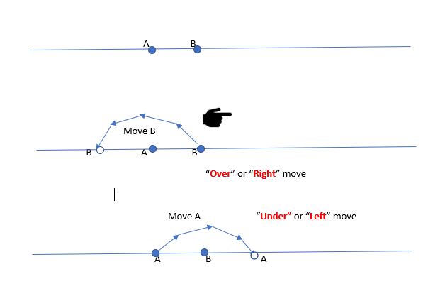
Another consequence of this work is obtained by generalizing the concept in this post to anyons, real particles in confined two-dimensional spaces. The analysis above speaks of exchange of particles. Anyons are a little more complex. You can exchange anyons by taking them “under” and also “over” as shown in the picture below.

These correspond to a change of sign of $\theta$ , so anyons can be represented by a combination of the commutators

$a b - e^{i \theta} b a = 1$

as well as

$a b - e^{-i \theta} b a = 1$

simultaneously. We therefore cannot think of $a$ and $b$ for an anyon (the lowering and raising operators) as matrices in the usual sense. They are much more complex objects!

Now, let’s consider two identical anyons propagating from a starting point to an ending point. If they were classical objects, they would just go and there would be one path connecting start to finish. But these are quantum objects! We need to sum over past histories, i.e., all the paths to go from the start to the finish. And when anyons travel, they could wind around each other. As in the figure below

Now, we sum over all the possible ways

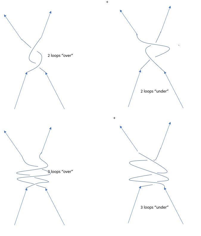
An amazing thing happens. If $\theta = 2 \pi \frac{M}{N}$ and $N$ were ${\bf even}$ , the sum over histories gives ${\bf 0}$ for the probability of propagation. ${\it Even-denominator \: anyons \: cannot \: propagate \: freely!}$ .

And here is the application – it is not easy to see the even – denominator fractional quantum Hall effect. The connection between the math and the quantum Hall effect is not transparent (from what I discussed above), but suffice it to say that the particles that give rise to the fractional quantum Hall effect are anyons and the fractions we obtain are exactly the fractions ( $\frac{M}{N}$ ) here. This geometrical observation “explains” the difficulty of observing the effect for even-denominator anyons.