Skip to content
Simply Curious
What is this blog about?
How I tried to build a crowd of AIs – and what it taught me about their shared mind
Ecuador, the Galápagos, and Peru: Notes from a Curious Traveler
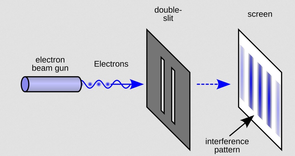
Measurement, Decoherence, and Why Quantum Outcomes Appear Stable
What’s the connection between spin and statistics – a simple argument
Why the Universe Isn’t Overflowing with Vacuum Energy: A Curious Field Theory Detour
The Great(er) American solar eclipse of 2024
Hawking radiation: a weight-loss program for black holes – another black hole conundrum and a cute connection between black holes and quantum field theory
Black hole conundrums – how to extract information from a black hole
1
2
3
…
7
Next Page
→
Subscribe
Subscribed
Simply Curious
Join 36 other subscribers
Sign me up
Already have a WordPress.com account?
Log in now.
Simply Curious
Subscribe
Subscribed
Sign up
Log in
Report this content
View site in Reader
Manage subscriptions
Collapse this bar